5  Collections

5.1 Introduction

In programming, there are occasions when we need a collection of items instead of just single values. For instance, to have names of all the students in a class we can create different variables and one by one assign students’ names to these variables. This would not only be a cumbersome process, for obvious reasons, but also would not serve the necessary future requirements such as new student enrollments or cancellation of enrolments. So, to cater to such situations where we need a collection and options to modify the collections as required, we use vectors. A vector is a data type that has one or more elements and there are functions to add and remove elements from a vector. The vectors are further classified as atomic vectors, lists, factors -- each of these data types offers some unique functionality. Let’s look into some examples for working with different types of vectors in R.

5.2 Vectors

The c function in the base package can be used to combine elements to create a vector or a list. A vector can have elements of one or more data types. A vector is mutable i.e. the we can add or remove elements in a vector. When combining numbers, the data type assigned the vector is numeric since the numbers can be with or without decimals. If the number are generated using the : operator then the resulting vector has integer data type.

nums <- c(1,2,3,4,5)
nums2 <- c(1:5)
cat(nums, class(nums),"\n")

1 2 3 4 5 numeric 

cat(nums2, class(nums2))

1 2 3 4 5 integer

chars1 <- c("hello", "world")
print(chars1)

[1] "hello" "world"

class(chars1)

[1] "character"

A vector can also be instantiated using a collection of variables; and these variables can be vectors as well. To get the count of number of elements in a vector, use the length function. Note that a vector has homogeneous data type i.e. all the elements in a vector has same data type. If you create a vectors with elements having different data types then the data types of some of the elements would be changed so that the resulting vectors is homogeneous - this process is called coercion.

name <- "Sam"
age <- 25

person1 <- c(name,age)
cat(person1, "\n")

Sam 25 

new_vec <- c(person1, person1)
cat(new_vec, "\n")

Sam 25 Sam 25 

cat(length(person1),length(new_vec),"\n")

2 4 

print(class(new_vec))

[1] "character"

The coercion is performed in the following order – logical integer double character. This means that the character data type gets the highest priority i.e. if in a vector, there is a combination of data types and at least one of the element is a character then all the elements would be coerced to character data type.

5.2.1 Naming elements in a vector

We can also give names to the elements of a vector as shown below. The vector elements can then be accessed by their names as well. The names can be given while declaring a vector directly or using setNames functions. The names can even be assigned after creating a vector. Notice that although the age variable is numeric, on creating a vector it is coerced to character data type. These names can then be used to access elements in a vector.

name <- "Sam"
age <- 25

person1<- c(name,age)

#Naming elements after creating a vector
names(person1) <- c("Name", "Age")

#Naming elements while initialing a vector
person2 <- c(Name = "Mike", Age = 30)
person3 <- setNames(c("Raj",35), c("Name","Age"))

print(person1)

 Name   Age 
"Sam"  "25" 

print(person2["Name"])

  Name 
"Mike" 

print(person3["Age"])

 Age 
"35" 

5.3 Lists

A list contains collection of elements and can be created using the list function. It looks similar to vectors but there are important differences between the two. A list can be heterogeneous i.e., unlike vectors, it can have elements of different data types.

new_list = list(1:5)
print(new_list)

[[1]]
[1] 1 2 3 4 5

print(class(new_list))

[1] "list"

In the output above, new_list is an object of the class list and has one element. It is important to note here that each element of a list is treated as a list itself. Therefore in the output above, [[1]] indicates the first element and double square brackets means that it is a list.

Another important difference between a vector and a list is that a list does not hold all the element rather it contains the reference to the elements. E.g. in the code below it may appear that the list has 6 elements - one string and five numbers. However, the length of list is 2. The first element is the string “hi” and the second element is a range of numbers from 1 to 5. Again, this is because each element of a list is essentially a list.

new_list2 = list("hi", 1:5)
print(new_list2)

[[1]]
[1] "hi"

[[2]]
[1] 1 2 3 4 5

print(length(new_list2))

[1] 2

To get a better sense of a list object we can use the str function to reveal its structure. Notice the two elements have different data types – lists are heterogeneous.

str(new_list2)

List of 2
 $ : chr "hi"
 $ : int [1:5] 1 2 3 4 5

We can access list elements by index (starting from 1) as well.

print(new_list2[2]) #print second element of the list.

[[1]]
[1] 1 2 3 4 5

A list element can have multiple lists. The code below creates a list have two elements each of which is a list. Note the indexing in the output — there are top level [[1]] and [[2]] referring to the two elements in the list_of_lists. Then we have [[1]][[1]] which refer to the first element of the first list and so on.

list_of_lists <- list(list(1:5,letters[1:5]), list(1:4,LETTERS[1:4]))
print(list_of_lists)

[[1]]
[[1]][[1]]
[1] 1 2 3 4 5

[[1]][[2]]
[1] "a" "b" "c" "d" "e"


[[2]]
[[2]][[1]]
[1] 1 2 3 4

[[2]][[2]]
[1] "A" "B" "C" "D"

cat('The length of the list_of_lists is ', length(list_of_lists))

The length of the list_of_lists is  2

When we look at the structure of list_of_lists, it shows the hierarchical organization of the list_of_lists wherein at the top there is a list of two elements and each element is a list of two elements. Let’s we want the second element of the first element from the list_of_lists (which is lower case characters) then we can use multi-indexing to get that element. We’ll first refer to the first element (which is a list) by [[1]] and then refer of its second element with [[2]].

str(list_of_lists)

List of 2
 $ :List of 2
  ..$ : int [1:5] 1 2 3 4 5
  ..$ : chr [1:5] "a" "b" "c" "d" ...
 $ :List of 2
  ..$ : int [1:4] 1 2 3 4
  ..$ : chr [1:4] "A" "B" "C" "D"

cat('The second element of first element is', list_of_lists[[1]][[2]])

The second element of first element is a b c d e

5.3.1 Naming elements in a list

Elements in a list can be assigned names (just like in the case of vectors). Elements in a named list can be accessed using the $ operator with the syntax <list name>$<element name>. Note that the setNames function returns a vector to change it to a list, as.list function can be used.

new_list2 = list("hi", 1:5)
names(new_list2) <- c("Text", "Numbers")
print(new_list2$Numbers)

[1] 1 2 3 4 5

student_list <- as.list(setNames(c("Raj",35), c("Name","Age")))
print(student_list$Name)

[1] "Raj"

5.4 Manipulating vectors and lists

Both vectors and lists are mutable data types i.e. the elements in these collections can be added or removed. To add an element, we can either directly add an element at a particular index or the append function can be used. When adding elements using index, if the index value is 1+ length(vector) then the element is added at the end of the vector. If the index value is greater than that then the new element is add at the index value and for the intervening values, NA is added. This method can also be used to replace and existing value a vector. By specifing a range as an index, we can also append a vector to a vector.

v1 <- c(1:5)
print(v1)

[1] 1 2 3 4 5

v1[6] <- 6
print(v1)

[1] 1 2 3 4 5 6

v1[8] <- 6
print(v1)

[1]  1  2  3  4  5  6 NA  6

v1[4] <- 6
print(v1)

[1]  1  2  3  6  5  6 NA  6

v1[9:11] <- c(7,8,9)
print(v1)

 [1]  1  2  3  6  5  6 NA  6  7  8  9

The append function takes two arguments - a vector or a list that is to be modified and a value that is to be added; it returns the modified vector. By default the value is appended at the end of the collection. To append at a desired index, a third argument (optional keyword — after) should be added and then the value is added after this index. We can, of course, append a vector to a vector.

v1 <- c(1:5)
v1 <- append(v1,6)
print(v1)

[1] 1 2 3 4 5 6

v1 <- append(v1,7,2)
print(v1)

[1] 1 2 7 3 4 5 6

v2 <- append(v1, c(8:10))
print(v2)

 [1]  1  2  7  3  4  5  6  8  9 10

student_list <- as.list(setNames(c("Raj",35), c("Name","Age")))
student_list <- append(student_list, 22)
print(student_list)

$Name
[1] "Raj"

$Age
[1] "35"

[[3]]
[1] 22

cat('The length of the list is ',length(student_list),'\n')

The length of the list is  3 

student_list[4] <- "Sam"
cat('The length of the list is ',length(student_list))

The length of the list is  4

5.5 Table 1: Comparison between a vector and a list

	Vector	List
Data type of elements	Homogeneous	Heterogeneous
coercion of data types	Yes	No
Structure	Contains individual elements	Each element of a list is essential a list itself.
Recursive	No	Yes, a list can contain list(s)
Length	Number of all the individual elements in the vector	Number of elements in the list but each element can itself be a list. So the length of a list may differ from the total elements contained in a list.

5.6 Factors

There is another variation of vectors which has some unique characteristics its called factor. It is used for working with categorical variables. Below, we create fruits as a factor having four element. When we print fruits we get the four elements as expected. What’s interesting is that a factor also has levels i.e. number of unique elements in the input vector.

fruits <- factor(c("apple", "mango", "banana", "apple"))
print(fruits)

[1] apple  mango  banana apple 
Levels: apple banana mango

To get the count of element for each of the level, table function is used.

table(fruits)

fruits
 apple banana  mango 
     2      1      1 

You may create your own levels and pass it to the factor. This is useful when the data has some fixed number of categories. This way when you tabulate a factor all the levels would be printed.

fruits_levels <- c("apple", "mango", "banana", "grapes")
levels(fruits) <- fruits_levels
table(fruits)

fruits
 apple  mango banana grapes 
     2      1      1      0 

Levels in factor ensure that no arbitrary data get in to a factor i.e. when we add an element to a factor that is not one of the levels then it is converted to NA.

fruits[5] <- "pineapple"

Warning in `[<-.factor`(`*tmp*`, 5, value = "pineapple"): invalid factor level,
NA generated

print(fruits)

[1] apple  banana mango  apple  <NA>  
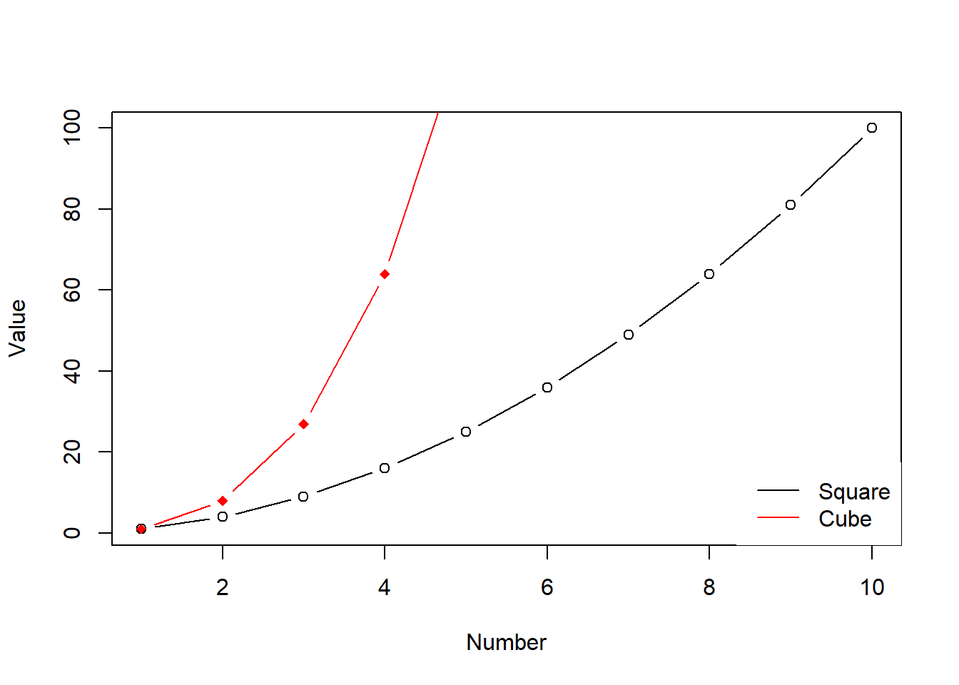
Levels: apple mango banana grapes

5.7 Plotting

The plot function provides a quick way to make graphs using data in vectors as a scatter plot. The lines function should be used to plot with lines.

x = c(1:10)
y = x**2
plot(x,y, xlab = "Number", ylab = "Value", type="b")
lines(x,x**3, xlab = "Number", ylab = "Value", type="b", col="red", pch=18)
legend("bottomright", legend = c("Square", "Cube"), col = c("black", "red"), lty=1, box.lty=0)